概要 誤差関数について理解する。
ガンマ関数について理解する。
単位階段関数について理解する。
デルタ関数について理解する。
双曲線関数について理解する。
誤差関数
奇関数である。
また、
e
r
f
c
(
t
)
=
1
−
e
r
f
(
t
)
{\displaystyle erfc(t)=1-erf(t)}
ガンマ関数
階乗の概念を一般化した関数である。
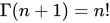
自然数nに対して、
Γ
(
n
+
1
)
=
n
!
{\displaystyle \Gamma (n+1)=n!}
単位階段関数
U
(
t
)
=
0
(
t
<
0
)
{\displaystyle U(t)=0(t<0)}
1
(
t
≥
0
)
{\displaystyle 1(t\geq 0)}
U
(
t
)
f
(
t
)
{\displaystyle U(t)f(t)}
t
<
0
{\displaystyle t<0}
0
{\displaystyle 0}
f
(
t
)
{\displaystyle f(t)}
デルタ関数
δ
(
t
)
=
0
(
t
≠
0
)
{\displaystyle \delta (t)=0\quad (t\neq 0)}
+
∞
(
t
=
0
)
{\displaystyle +\infty \quad (t=0)}
t
=
0
{\displaystyle t=0}
双曲線関数
sinh
(
a
x
)
=
e
a
x
−
e
−
a
x
2
{\displaystyle \sinh(ax)={\frac {e^{ax}-e^{-ax}}{2}}}
cosh
(
a
x
)
=
e
a
x
+
e
−
a
x
2
{\displaystyle \cosh(ax)={\frac {e^{ax}+e^{-ax}}{2}}}
tanh
(
a
x
)
=
e
a
x
−
e
−
a
x
e
a
x
+
e
−
a
x
{\displaystyle \tanh(ax)={\frac {e^{ax}-e^{-ax}}{e^{ax}+e^{-ax}}}}
特殊関数とは 特殊関数(special functions)とは、特定の分野で何らかの名前や記法が定着している関数のことを指す。
ラプラス変換で扱う特殊関数
ラプラス変換では、以下のような特殊関数を扱う。 誤差関数(ガウスの誤差関数)
ガンマ関数(オイラーのガンマ関数)
単位階段関数(ヘビサイドの単位階段関数)
デルタ関数(ディラクの衝撃関数)
誤差関数 定義1:
以下の式で定義された関数erf(t)を誤差関数(error function)という。
e
r
f
(
t
)
=
2
π
∫
0
t
e
−
x
2
d
x
{\displaystyle erf(t)={\frac {2}{\sqrt {\pi }}}\int _{0}^{t}{e^{-x^{2}}\,dx}}
e
r
f
c
(
t
)
=
1
−
e
r
f
(
t
)
{\displaystyle erfc(t)=1-erf(t)}
図. 誤差関数のグラフ
e
r
f
(
a
σ
2
)
{\displaystyle erf\left({\frac {a}{\sigma {\sqrt {2}}}}\right)}
誤差関数は奇関数である。
測定値が正規分布になっていて、標準偏差が
σ
{\displaystyle \sigma }
0
{\displaystyle 0}
−
a
{\displaystyle -a}
a
{\displaystyle a}
ガンマ関数 定義:
以下の無限積分で定義された関数
Γ
(
p
)
{\displaystyle \Gamma (p)}
Γ
(
p
)
=
∫
0
+
∞
x
p
−
1
e
−
x
d
x
(
p
>
0
)
{\displaystyle \Gamma (p)=\int _{0}^{+\infty }{x^{p-1}\,e^{-x}\,dx}\qquad (p>0)}
Γ
(
p
)
{\displaystyle \Gamma (p)}
p
{\displaystyle p}
p
{\displaystyle p}
図. ガンマ関数のグラフ
n
{\displaystyle n}
Γ
(
n
+
1
)
=
n
!
{\displaystyle \Gamma (n+1)=n!}
n
!
=
n
(
n
−
1
)
(
n
−
2
)
.
.
.
3
⋅
2
⋅
1
(
n
:
正 の 整 数
)
{\displaystyle n!=n(n-1)(n-2)\,...\,3\cdot 2\cdot 1\qquad (n:{\mbox{ 正 の 整 数 }})}
ガンマ関数の性質
Γ
(
p
+
1
)
=
p
Γ
(
p
)
(
p
>
0
)
{\displaystyle \Gamma (p+1)=p\Gamma (p)\qquad (p>0)}
p
=
n
−
1
{\displaystyle p=n-1}
Γ
(
n
)
=
(
n
−
1
)
Γ
(
n
−
1
)
{\displaystyle \Gamma (n)=(n-1)\Gamma (n-1)}
Γ
(
1
)
=
1
{\displaystyle \Gamma (1)=1}
Γ
(
n
)
=
(
n
−
1
)
!
(
n
=
2
,
3
,
4
,
⋯
)
{\displaystyle \Gamma (n)=(n-1)!\qquad (n=2,3,4,\cdots )}
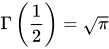
Γ
(
1
2
)
=
π
{\displaystyle \Gamma \left({\frac {1}{2}}\right)={\sqrt {\pi }}}
Γ
(
n
2
)
=
(
π
2
m
)
(
2
m
−
1
)
(
2
m
−
3
)
⋯
3
⋅
1
(
m
,
n
:
正 整 数
,
n
=
2
m
+
1
:
奇 数
)
{\displaystyle \Gamma \left({\frac {n}{2}}\right)=\left({\frac {\sqrt {\pi }}{2^{m}}}\right)\,(2m-1)\,(2m-3)\,\cdots 3\cdot 1\qquad (m,n:{\mbox{ 正 整 数 }},\,n=2m+1:{\mbox{ 奇 数 }})}
式
Γ
(
p
+
1
)
=
p
Γ
(
p
)
{\displaystyle \Gamma (p+1)=p\Gamma (p)}
p
<
0
{\displaystyle p<0}
Γ
(
p
)
{\displaystyle \Gamma (p)}
図. 定義域を拡張したガンマ関数のグラフ
例題:
以下のガンマ関数の値を求めよ。
(1)
Γ
(
3
)
{\displaystyle \Gamma (3)}
Γ
(
3
2
)
{\displaystyle \Gamma \left({\frac {3}{2}}\right)}
Γ
(
3
)
=
(
3
−
1
)
!
=
2
{\displaystyle \Gamma (3)=(3-1)!=2}
Γ
(
3
2
)
=
(
3
2
−
1
)
Γ
(
3
2
−
1
)
=
1
2
Γ
(
1
2
)
=
π
2
{\displaystyle {\begin{aligned}\Gamma \left({\frac {3}{2}}\right)&=\left({\frac {3}{2}}-1\right)\,\Gamma \left({\frac {3}{2}}-1\right)\\&={\frac {1}{2}}\,\Gamma \left({\frac {1}{2}}\right)\\&={\frac {\sqrt {\pi }}{2}}\end{aligned}}}
単位階段関数 定義:
以下で定義された関数U(t)を単位階段関数(unit step function)という。
U
(
t
)
=
{
0
(
t
<
0
)
1
(
t
≥
0
)
{\displaystyle U(t)={\begin{cases}0&\qquad (t<0)\\1&\qquad (t\geq 0)\end{cases}}}
t
=
0
{\displaystyle t=0}
t
=
0
{\displaystyle t=0}
図. 単位階段関数のグラフ
U
(
t
)
{\displaystyle U(t)}
t
{\displaystyle t}
t
=
0
{\displaystyle t=0}
f
(
t
)
{\displaystyle f(t)}
U
(
t
)
f
(
t
)
{\displaystyle U(t)f(t)}
t
=
a
{\displaystyle t=a}
U
(
t
)
f
(
t
)
{\displaystyle U(t)f(t)}
U
(
t
−
a
)
f
(
t
−
a
)
{\displaystyle U(t-a)f(t-a)}
図.
U
(
t
)
f
(
t
)
{\displaystyle U(t)f(t)}
t
=
0
{\displaystyle t=0}
f
(
t
)
{\displaystyle f(t)}
y
=
U
(
t
)
sin
t
{\displaystyle y=U(t)\,\sin {t}}
y
=
U
(
t
)
sin
t
{\displaystyle y=U(t)\,\sin {t}}
U
(
t
)
{\displaystyle U(t)}
t
<
0
{\displaystyle t<0}
0
{\displaystyle 0}
図.
y
=
U
(
t
)
sin
t
{\displaystyle y=U(t)\,\sin {t}}
デルタ関数 定義:
以下の式で表される関数δ(t)を、デルタ関数(delta function)という。
δ
(
t
)
=
{
0
(
t
≠
0
)
+
∞
(
t
=
0
)
{\displaystyle \delta (t)={\begin{cases}0&\quad (t\neq 0)\\+\infty &\quad (t=0)\end{cases}}}
∫
−
∞
+
∞
δ
(
t
)
d
t
=
1
{\displaystyle \int _{-\infty }^{+\infty }{\delta (t)\,dt}=1}
図. デルタ関数のグラフ
∑
n
=
0
∞
δ
(
t
−
n
a
)
(
n
:
自 然 数
)
{\displaystyle \sum _{n=0}^{\infty }{\delta (t-na)}\qquad (n:{\mbox{ 自 然 数 }})}
図.
t
=
a
,
2
a
,
3
a
,
.
.
.
(
a
≥
0
)
{\displaystyle t=a,\,2a,\,3a,\,...\quad (a\geq 0)}
デルタ関数の性質構文解析に失敗 (Conversion error. Server ("https://wikimedia.org/api/rest_") reported: "Cannot get mml. Server problem."): {\displaystyle \delta (x-a)={\frac {d}{dx}}\,U(x-a)}
∫
−
∞
+
∞
f
(
x
)
δ
(
x
−
a
)
=
f
(
a
)
{\displaystyle \int _{-\infty }^{+\infty }{f(x)\,\delta (x-a)}=f(a)}
x
δ
(
x
−
a
)
=
a
δ
(
x
−
a
)
{\displaystyle x\,\delta (x-a)=a\,\delta (x-a)}
f
(
x
)
δ
(
x
−
a
)
=
f
(
a
)
δ
(
x
−
a
)
{\displaystyle f(x)\,\delta (x-a)=f(a)\,\delta (x-a)}
双曲線関数 双曲線関数の概要 以下に示す2つの指数関数を組み合わせることによって作られる関数を考える。
構文解析に失敗 (Conversion error. Server ("https://wikimedia.org/api/rest_") reported: "Cannot get mml. Server problem."): {\displaystyle y=e^{ax}</math*<math>y=e^{-ax}\qquad (a\neq 0)}
sinh
(
a
x
)
=
e
a
x
−
e
−
a
x
2
{\displaystyle \sinh(ax)={\frac {e^{ax}-e^{-ax}}{2}}}
cosh
(
a
x
)
=
e
a
x
+
e
−
a
x
2
{\displaystyle \cosh(ax)={\frac {e^{ax}+e^{-ax}}{2}}}
tanh
(
a
x
)
=
e
a
x
−
e
−
a
x
e
a
x
+
e
−
a
x
{\displaystyle \tanh(ax)={\frac {e^{ax}-e^{-ax}}{e^{ax}+e^{-ax}}}}
sinh
(
a
x
)
,
cosh
(
a
x
)
,
tanh
(
a
x
)
{\displaystyle \sinh(ax),\,\cosh(ax),\,\tanh(ax)}
sin
(
a
x
)
,
cos
(
a
x
)
,
tan
(
a
x
)
{\displaystyle \sin(ax),\,\cos(ax),\,\tan(ax)}
構文解析に失敗 (Conversion error. Server ("https://wikimedia.org/api/rest_") reported: "Cannot get mml. Server problem."): {\displaystyle \cosh(ax)}
は、懸垂曲線(カテナリー, catenary)とも呼ばれる。
e
x
=
cosh
(
x
)
+
sinh
(
x
)
{\displaystyle e^{x}=\cosh(x)+\sinh(x)}
e
−
x
=
cosh
(
x
)
−
sinh
(
x
)
{\displaystyle e^{-x}=\cosh(x)-\sinh(x)}
cosh
(
x
)
,
sinh
(
x
)
{\displaystyle \cosh(x),\,\sinh(x)}
構文解析に失敗 (Conversion error. Server ("https://wikimedia.org/api/rest_") reported: "Cannot get mml. Server problem."): {\displaystyle x^{2}-y^{2}=1}
上の点である。
cosh
2
(
x
)
−
sinh
2
(
x
)
=
1
{\displaystyle \cosh ^{2}(x)-\sinh ^{2}(x)=1}
双曲線関数の性質 (1)
cosh
2
(
a
x
)
−
sinh
2
(
a
x
)
=
1
{\displaystyle \cosh ^{2}(ax)-\sinh ^{2}(ax)=1}
tanh
(
a
x
)
=
sinh
(
a
x
)
cosh
(
a
x
)
{\displaystyle \tanh(ax)={\frac {\sinh(ax)}{\cosh(ax)}}}
構文解析に失敗 (Conversion error. Server ("https://wikimedia.org/api/rest_") reported: "Cannot get mml. Server problem."): {\displaystyle \sinh(x\pm y)=\sinh(x)\cosh(y)\pm \cosh(x)\sinh(y)}
(4)
cosh
(
x
±
y
)
=
cosh
(
x
)
cosh
(
y
)
±
sinh
(
x
)
sinh
(
y
)
{\displaystyle \cosh(x\pm y)=\cosh(x)\cosh(y)\pm \sinh(x)\sinh(y)}
tanh
(
x
±
y
)
=
tanh
(
x
)
±
tanh
(
y
)
1
±
tanh
(
x
)
tanh
(
y
)
{\displaystyle \tanh(x\pm y)={\frac {\tanh(x)\pm \tanh(y)}{1\pm \tanh(x)\tanh(y)}}}
双曲線関数の微分:
(1)
d
d
x
sinh
(
a
x
)
=
a
cosh
(
a
x
)
{\displaystyle {\frac {d}{dx}}\,\sinh(ax)=a\cosh(ax)}
構文解析に失敗 (Conversion error. Server ("https://wikimedia.org/api/rest_") reported: "Cannot get mml. Server problem."): {\displaystyle {\frac {d}{dx}}\,\cosh(ax)=a\sinh(ax)}
双曲線関数の積分:
(1)
∫
sinh
(
a
x
)
d
x
=
cosh
(
a
x
)
a
+
C
{\displaystyle \int {\sinh(ax)\,dx}={\frac {\cosh(ax)}{a}}+C}
∫
cosh
(
a
x
)
d
x
=
sinh
(
a
x
)
a
+
C
{\displaystyle \int {\cosh(ax)\,dx}={\frac {\sinh(ax)}{a}}+C}
双曲線関数の例題 例題:
双曲線関数の定義に基づいて以下が成立することを示せ。
d
d
x
sinh
(
a
x
)
=
a
cosh
(
a
x
)
{\displaystyle {\frac {d}{dx}}\sinh(ax)=a\cosh(ax)}
構文解析に失敗 (Conversion error. Server ("https://wikimedia.org/api/rest_") reported: "Cannot get mml. Server problem."): {\displaystyle {\begin{aligned}{\frac {d}{dx}}\sinh(ax)&={\frac {d}{dx}}\,{\frac {e^{ax}-e^{-ax}}{2}}\\&={\frac {ae^{ax}-(-a)e^{-ax}}{2}}\\&={\frac {a(e^{ax}+e^{-ax})}{2}}\\&=a\cosh(ax)\end{aligned}}}